Introduction

Before diving into the core tutorial, it is important to understand that OpenGL has evolved over the years and a big change occured in 2003 with the introduction of the dynamic pipeline (OpenGL 2.0), i.e. the use of shaders that allow to have direct access to the GPU.

Note

ES is a light version of OpenGL for embedded systems such as tablets or mobiles. There also exists WebGL which is very similar to ES but is not shown on this graphic.

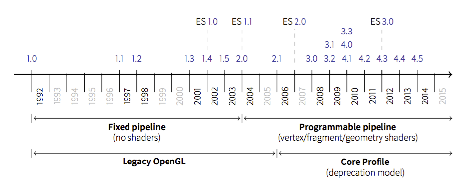
Before this version, OpenGL was using a fixed pipeline and you may still find a lot of tutorials that still use this fixed pipeline. How to know if a tutorial address the fixed pipeline ? It’s relatively easy. If you see GL commands such as:

glVertex, glColor, glLight, glMaterial
glBegin, glEnd
glMatrix, glMatrixMode, glLoadIdentity
glPushMatrix, glPopMatrix
glRect, glPolygonMode
glBitmap, glAphaFunc
glNewList, glDisplayList
glPushAttrib, glPopAttrib
glVertexPointer, glColorPointer, glTexCoordPointer, glNormalPointer

then it’s most certainly a tutorial that adress the fixed pipeline. While modern OpenGL is far more powerful than the fixed pipeline version, the learning curve may be a bit steeper. This tutorial will try to help you start using it.

Program and shaders

Note

The shader language is called glsl. There are many versions that goes from 1.0 to 1.5 and subsequents version get the number of OpenGL version. Last version is 4.4 (February 2014).

Shaders are pieces of program (using a C-like language) that are build onto the GPU and executed during the rendering pipeline. Depending on the nature of the shaders (there are many types depending on the version of OpenGL you’re using), they will act at different stage of the rendering pipeline. To simplify this tutorial, we’ll use only vertex and fragment shader as shown below:

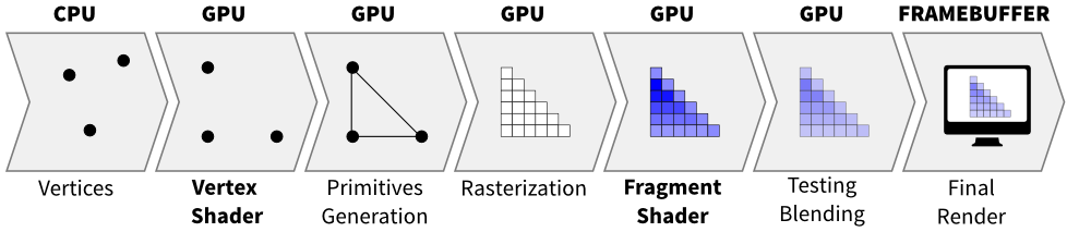
A vertex shader acts on vertices and is supposed to output the vertex position (→ gl_Position) on the viewport (i.e. screen). A fragment shader acts at the fragment level and is supposed to output the color (→ gl_FragColor) of the fragment. Hence, a minimal vertex shader is:

void main()
{
    gl_Position = vec4(0.0,0.0,0.0,1.0);
}

while a minimal fragment shader would be:

void main()
{
    gl_FragColor = vec4(0.0,0.0,0.0,1.0);
}

These two shaders are not very useful since the first will transform any vertex into the null vertex while the second will output the black color for any fragment. We’ll see later how to make them to do more useful things.

One question remains: when are those shaders exectuted exactly ? The vertex shader is executed for each vertex that is given to the rendering pipeline (we’ll see what does that mean exactly later) and the fragment shader is executed on each fragment that is generated after the vertex stage. For example, in the simple figure above, the vertex would be called 3 times, once for each vertex (1,2 and 3) while the fragment shader would be executed 21 times, once for each fragment (pixel).

Buffers and textures

We explained earlier that the vertex shader act on the vertices. The question is thus where do those vertices comes from ? The idea of modern GL is that vertices are stored on the GPU and needs to be uploaded (only once) to the GPU before rendering. The way to do that is to build buffers onto the CPU and to send them onto the GPU. If your data does not change, no need to upload it again. That is the big difference with the previous fixed pipeline where data were uploaded at each rendering call (only display lists were built into GPU memory).

But what is the structure of a vertex ? OpenGL does not assume anything about your vertex structure and you’re free to use as many information you may need for each vertex. The only condition is that all vertices from a buffer have the same structure (possibly with different content). This again is a big difference with the fixed pipeline where OpenGL was doing a lot of complex rendering stuff for you (projections, lighting, normals, etc.) with an implicit fixed vertex structure. Now you’re on your own…

Good news is that you’re now free to do anything you want.

Bad news is that you have to program everything.

Let’s take a simple example of a vertex structure where we want each vertex to hold a position and a color. The easiest way to do that in python is to use a structured array using the numpy library:

data = numpy.zeros(4, dtype = [ ("position", np.float32, 3),
                                ("color",    np.float32, 4)] )

We just created a CPU buffer with 4 vertices, each of them having a position (3 floats for x,y,z coordinates) and a color (4 floats for red, blue, green and alpha channels). Note that we explicitely chose to have 3 coordinates for position but we may have chosen to have only 2 if were to work in two-dimensions only. Same holds true for color. We could have used only 3 channels (r,g,b) if we did not want to use transparency. This would save some bytes for each vertex. Of course, for 4 vertices, this does not really matter but you have to realize it will matter if you data size grows up to one or ten million vertices.

Variables

At this point in the tutorial, we know what are shaders and buffers but we still need to explain how they may be connected together. So, let’s consider again our CPU buffer:

data = numpy.zeros(4, dtype = [ ("position", np.float32, 2),
                                ("color",    np.float32, 4)] )

We need to tell the vertex shader that it will have to handle vertices where a position is a tuple of 2 floats and color is a tuple of 4 floats. This is precisely what attributes are meant for. Let us change slightly our previous vertex shader:

attribute vec2 position;
attribute vec4 color;
void main()
{
    gl_Position = vec4(position, 0.0, 1.0);
}

This vertex shader now expects a vertex to possess 2 attributes, one named position and one named color with specified types (vec3 means tuple of 3 floats and vec4 means tuple of 4 floats). It is important to note that even if we labeled the first attribute position, this attribute is not yet bound to the actual position in the numpy array. We’ll need to do it explicitly at some point in our program and there is no automagic that will bind the numpy array field to the right attribute, you’ll have to do it yourself, but we’ll see that later.

The second type of information we can feed the vertex shader are the uniforms that may be considered as constant values (across all the vertices). Let’s say for example we want to scale all the vertices by a constant factor scale, we would thus write:

uniform float scale;
attribute vec2 position;
attribute vec4 color;
void main()
{
    gl_Position = vec4(position*scale, 0.0, 1.0);
}

Last type is the varying type that is used to pass information between the vertex stage and the fragment stage. So let us suppose (again) we want to pass the vertex color to the fragment shader, we now write:

uniform float scale;
attribute vec2 position;
attribute vec4 color;
varying vec4 v_color;

void main()
{
    gl_Position = vec4(position*scale, 0.0, 1.0);
    v_color = color;
}

and then in the fragment shader, we write:

varying vec4 v_color;

void main()
{
    gl_FragColor = v_color;
}

The question is what is the value of v_color inside the fragment shader ? If you look at the figure that introduced the gl pipleline, we have 3 vertices and 21 fragments. What is the color of each individual fragment ?

The answer is the interpolation of all 3 vertices color. This interpolation is made using distance of the fragment to each individual vertex. This is a very important concept to understand. Any varying value is interpolated between the vertices that compose the elementary item (mostly, line or triangle).